Decision Trees

Author

Daniel Redel

Published

March 30, 2024

import numpy as np
import pandas as pd
import matplotlib.pyplot as plt
import seaborn as sns

import warnings
warnings.filterwarnings("ignore")

Decision trees are nonlinear graphical models that have found important applications in machine learning mainly due to their interpretability as well as their roles in other powerful models such as random forests and gradient boosting regression trees that we will see in the next section.

Decision Trees involve segmenting the predictor space \textbf{X} into a number of simple rectangular regions. Unlike linear models that result in linear decision boundaries, decision trees partition the feature space into hyper-rectangular decision regions and, therefore, they are nonlinear models.

In this chapter we describe the principles behind training a popular type of decision trees known as CART (short for Classification and Regression Tree).

Regression Trees

A regression tree consists of a series of splitting rules, starting at the top of the tree. Roughly speaking, there are two steps:

We divide the predictor space —set of possible values for X_1, X_2,...,X_p — into J distinct and non-overlapping regions, R_1, R_2,...,R_J.
For every observation that falls into the region R_j, we make the same prediction, which simply the mean of the response values for the training observations in R_j.

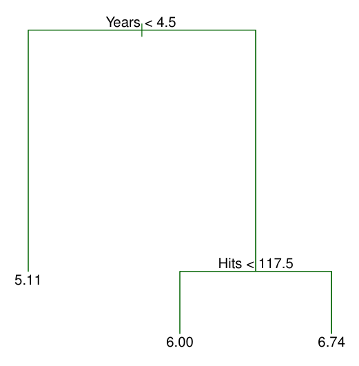
In this example, The top split assigns observations having Years<4.5 to the left branch. This first region can be written as R_1=(X|\text{Years<4.5}).

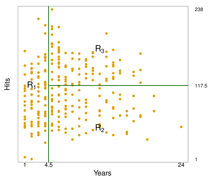
The regions R_1, R_2, and R_3 are known as terminal nodes or leaves of the tree.
The points along the tree where the predictor space is split are referred to as internal nodes.
At a given internal node, the label of the form X_j < t_k indicates the left-hand branch emanating from that split, and the right-hand branch corresponds to X_j ≥ t_k.

Recursive Binnary Splitting

How do we construct the regions R_1,...,R_J? The goal is to find boxes R_1,...,R_J that minimize the \text{RSS}, given by

\sum^J_{j=1}\sum_{i \in R_j} (y_i-\hat{y}_{R_j})^2

where \hat{y}_{R_j} is the mean response within the j th box.

Unfortunately, it is computationally infeasible to consider every possible partition of the feature space into J boxes.

💡 For this reason, we take a top-down, greedy approach that is known as recursive binary splitting.

Top-Down: The approach is top-down because it begins at the top of the tree and then successively splits the predictor space; each split is indicated via two new branches further down on the tree.
Greedy: It is greedy because at each step of the tree-building process, the best split is made at that particular step, rather than looking ahead and picking a split that will lead to a better tree in some future step.

Because we do this sequential for every internal node, the algorithm is called recursive binary splitting.

Step 1: Select X_j and s (Find partitions) that leads to greatest reduction in \text{RSS}

In order to perform recursive binary splitting, we first select the predictor X_j and the cutpoint s such that splitting the predictor space into the regions (X|X_j<s) and (X|X_j\geq s) leads to the greatest possible reduction in \text{RSS}.
The notation (X|X_j<s) means the Region R_1(j,s) of predictor space in which X_j takes on a value less than s. Thus, we choose the predictor X_j and cutpoint s such that the resulting tree has the lowest RSS.

Step 2: Select X_j and s that leads to even greatest reduction in \text{RSS} within each of the already identified regions.

Next, we repeat the process, looking for the best predictor X_j and best cutpoint s in order to split the data further so as to minimize the \text{RSS} within each of the resulting regions.

Step 3: The process continues until a stopping criterion is reached.

For instance, we may continue until no region contains more than 5 observations.

Step 4: Predict Responses in Test Sample.

Once the regions R_1,...,R_J have been created, we predict the response for a given test observation using the mean of the training observations in the region to which that test observation belongs.

Tree Prunning

Challenge: good predictions on the training set, but likely to overfit the data, leading to poor test set performance. This is because the resulting tree might be too complex. A smaller tree with fewer splits might lead to lower variance and better interpretation at the cost of a little bias.

Solution: Therefore, a better strategy is to grow a very large tree T_0, and then prune it back in order to obtain a subtree(Backward Stepwise).

Cost Complexity Pruning: Rather than considering every possible subtree, we consider a sequence of trees indexed by a nonnegative tuning parameter α. For each value of \alpha there corresponds a subtree T\in T_0 such that:

\sum^{\lvert T \rvert}_{M=1}\sum_{i:x_i\in R_m}(y_i-\hat{y}_{R_m})^2+a\lvert T \rvert

is as small as possible.

Here \lvert T\rvert indicates the number of terminal nodes of the tree T
R_m is the rectangle (the subset of predictor space) corresponding to the m th terminal node, and \hat{y}_{R_m} is the predicted response associated with R_m—that is, the mean of the training observations in R_m.

💡 The tuning parameter α controls a trade-off between the subtree’s complexity and its fit to the training data.

When α = 0, then the subtree T=T_0.
As α increases, there is a price to pay for having a tree with many terminal nodes.

💡 We can select a value of α using a validation set or using cross-validation. We then return to the full data set and obtain the subtree corresponding to α.

Model Training

Here we fit a regression tree to the Boston data set. The steps are similar to those for classification trees.

Code

from ISLP import load_data, confusion_table
df = load_data("Boston")

df.head(5)

Table 1: Boston Dataset

	crim	zn	indus	nox	rm	age	dis	rad	tax	ptratio	lstat	medv
0	0.00632	18.0	2.31	0.538	6.575	65.2	4.0900	1	296	15.3	4.98	24.0
1	0.02731	0.0	7.07	0.469	6.421	78.9	4.9671	2	242	17.8	9.14	21.6
2	0.02729	0.0	7.07	0.469	7.185	61.1	4.9671	2	242	17.8	4.03	34.7
3	0.03237	0.0	2.18	0.458	6.998	45.8	6.0622	3	222	18.7	2.94	33.4
4	0.06905	0.0	2.18	0.458	7.147	54.2	6.0622	3	222	18.7	5.33	36.2

from sklearn.model_selection import train_test_split
from sklearn.preprocessing import StandardScaler
from sklearn.tree import DecisionTreeRegressor as DT

# Target vs Inputs
X = df.drop(columns=["medv"]) # Covariates-Only
y = df["medv"] # Target-Outcome

# Train vs Split
X_train, X_test, y_train, y_test = train_test_split(X, y, test_size=0.2, random_state=0)

# Initialize Decision Tree Regressor
dtree = DT(random_state=0)

# Train Model
dtree.fit(X_train, y_train)

# Predict
y_test_pred = dtree.predict(X_test)

Code

from sklearn import tree
my_tree = tree.plot_tree(dtree, filled=True)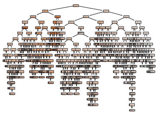

from sklearn.metrics import accuracy_score, mean_squared_error
print('R2 Train' , dtree.score(X_train, y_train).round(2) ) 
print('R2 Test' , dtree.score(X_test, y_test).round(2) ) 
print( 'Test MSE:', mean_squared_error(y_test, y_test_pred).round(2) )

R2 Train 1.0
R2 Test 0.58
Test MSE: 34.04

As expected, the accuracy on the training set is 100% —because the leaves are pure, the tree was grown deep enough that it could perfectly memorize all the labels on the training data. The test set accuracy is a lot worse than for the linear models we looked at previously, which had around 58% accuracy.

Unpruned trees are therefore prone to overfitting and not generalizing well to new data. Now let’s apply pruning to the tree.

Tree Pruning

We use the full tree we already built (dtree) to then run the cost_complexity_pruning_path() method of dtree to extract cost-complexity values:

import sklearn.model_selection as skm

ccp_path = dtree.cost_complexity_pruning_path(X_train, y_train)
kfold = skm.KFold(5, shuffle=True, random_state=10)

Optimal Alpha: -15.28

This yields a set of impurities and \alpha values from which we can extract an optimal one by cross-validation (GridSearchCV):

# Grid Search
grid = skm.GridSearchCV(dtree, {'ccp_alpha': ccp_path.ccp_alphas}, refit=True, cv=kfold, scoring='neg_mean_squared_error')

# Fit Model
G = grid.fit(X_train, y_train)

# Best
best_ = grid.best_estimator_

print('Optimal Alpha:', grid.best_score_.round(2))

Let’s plot the best tree to see how interpretable it is now:

Code

from sklearn import tree
column_names = X.columns.tolist()

best_ = G.best_estimator_
my_tree = tree.plot_tree(best_, feature_names=column_names, filled=True)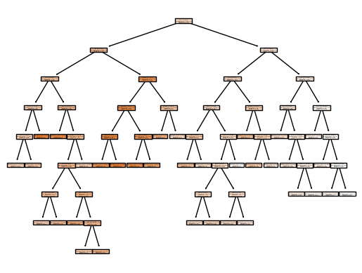

In keeping with the cross-validation results, we use the pruned tree to make predictions on the test set:

from sklearn.metrics import accuracy_score, mean_squared_error
print('R2 Train' , best_.score(X_train, y_train).round(2) ) 
print('R2 Test' , best_.score(X_test, y_test).round(2) ) 
print( 'Test MSE:', mean_squared_error(y_test, best_.predict(X_test)).round(2) )

R2 Train 0.95
R2 Test 0.61
Test MSE: 31.83

In other words, the test set MSE associated with the regression tree is 31.8. Prunning the tree decreases overfitting. This leads to a lower accuracy on the training set, but an improvement on the test set.

Feature Importance

feat_importance = best_.tree_.compute_feature_importances(normalize=False)
column_names = X.columns.tolist()
fimp_df = pd.DataFrame(feat_importance, column_names).reset_index().sort_values(0, ascending=False).head(10)

Code

fig, ax = plt.subplots()

# Setup
data = fimp_df.loc[:,0].sort_values()
index = np.arange(data.shape[0])
bar_labels = fimp_df.sort_values(0).loc[:,'index'].tolist()
bar_colors = ['#F2F299', '#C8E29D', '#5E9387', '#58828B']
bar_width = 0.9

# Figure
ax.barh(index, data, bar_width, label=bar_labels, color=bar_colors)

# Labels
ax.set_ylabel('Feature Importance')
ax.set_yticks(index, labels=bar_labels)

# Show
plt.show()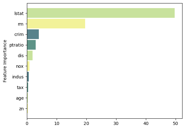

Figure 3: Feature Importance Classification Tree

Classification Trees

For a classification tree, we predict that each observation belongs to the most commonly occurring class of training observations in the region to which it belongs.

Just as in the regression setting, we use recursive binary splitting to grow a classification tree.

However, in the classification setting, RSS cannot be used as a criterion for making the binary splits. So, we need to find another Impurity Measure for classification problems.

Impurity Measures

There are some common measures of impurity that satisfy these requirements. Common choices include Gini, Entropy, and Misclassification Error (if we classify all observations in S to the majority class) given by:

\text{Gini Index: } G=\sum^K_{k=1} \hat{p}_{mk}(1-\hat{p}_{mk}) \\ \text{Entropy: } D=-\sum^K_{k=1} \hat{p}_{mk}\log(\hat{p}_{mk}) \\ \text{Error Rate: } E=1-\max_k(\hat{p}_{mk})

In fact, it turns out that the Gini index and the entropy are quite similar numerically. When building a classification tree, either the Gini index or the entropy are typically used to evaluate the quality of a particular split, since these two approaches are more sensitive to node purity than is the classification error rate.

Model Training

Code

from sklearn.datasets import load_breast_cancer
cancer = load_breast_cancer()

df = pd.DataFrame(cancer.data, columns=cancer.feature_names)
# Add target
df['target'] = cancer.target

df.head(5)

Table 2: Breast Cancer Dataset

	mean radius	mean texture	mean perimeter	mean area	mean smoothness	mean compactness	mean concavity	mean concave points	mean symmetry	mean fractal dimension	...	worst texture	worst perimeter	worst area	worst smoothness	worst compactness	worst concavity	worst concave points	worst symmetry	worst fractal dimension
0	17.99	10.38	122.80	1001.0	0.11840	0.27760	0.3001	0.14710	0.2419	0.07871	...	17.33	184.60	2019.0	0.1622	0.6656	0.7119	0.2654	0.4601	0.11890
1	20.57	17.77	132.90	1326.0	0.08474	0.07864	0.0869	0.07017	0.1812	0.05667	...	23.41	158.80	1956.0	0.1238	0.1866	0.2416	0.1860	0.2750	0.08902
2	19.69	21.25	130.00	1203.0	0.10960	0.15990	0.1974	0.12790	0.2069	0.05999	...	25.53	152.50	1709.0	0.1444	0.4245	0.4504	0.2430	0.3613	0.08758
3	11.42	20.38	77.58	386.1	0.14250	0.28390	0.2414	0.10520	0.2597	0.09744	...	26.50	98.87	567.7	0.2098	0.8663	0.6869	0.2575	0.6638	0.17300
4	20.29	14.34	135.10	1297.0	0.10030	0.13280	0.1980	0.10430	0.1809	0.05883	...	16.67	152.20	1575.0	0.1374	0.2050	0.4000	0.1625	0.2364	0.07678

5 rows × 31 columns

from sklearn.model_selection import train_test_split
from sklearn.preprocessing import StandardScaler
from sklearn.tree import DecisionTreeClassifier as DT

# Target vs Inputs
X = df.drop(columns=["target"]) # Covariates-Only
y = df["target"] # Target-Outcome

# Train vs Split
X_train, X_test, y_train, y_test = train_test_split(X, y, test_size=0.2, random_state=0)

# Initialize Decision Tree Regressor
dtree = DT(random_state=0)

# Train Model
dtree.fit(X_train, y_train)

# Predict
y_test_pred = dtree.predict(X_test)

Code

from sklearn import tree
my_tree = tree.plot_tree(dtree, filled=True)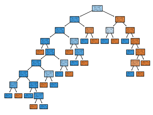

from sklearn.metrics import accuracy_score, mean_squared_error
print('R2 Train' , dtree.score(X_train, y_train).round(2) ) 
print('R2 Test' , dtree.score(X_test, y_test).round(2) ) 
print( 'Test MSE:', mean_squared_error(y_test, y_test_pred).round(2) )

R2 Train 1.0
R2 Test 0.91
Test MSE: 0.09

Tree Prunning

We first refit the full tree on the training set; here we do not set a max_depth parameter, since we will learn that through cross-validation.

from sklearn.model_selection import train_test_split
from sklearn.preprocessing import StandardScaler
from sklearn.tree import DecisionTreeClassifier as DT

# Train vs Split
X_train, X_test, y_train, y_test = train_test_split(X, y, test_size=0.2, random_state=0)

# Initialize Decision Tree Regressor
dtree = DT(random_state=0)

# Train Model
dtree.fit(X_train, y_train)

# Predict
y_test_pred = dtree.predict(X_test)

Next we use the cost_complexity_pruning_path() method of dtree to extract cost-complexity values:

import sklearn.model_selection as skm

ccp_path = dtree.cost_complexity_pruning_path(X_train, y_train)
kfold = skm.KFold(10, random_state=1, shuffle=True)

This yields a set of impurities and \alpha values from which we can extract an optimal one by cross-validation (GridSearchCV):

grid = skm.GridSearchCV(dtree,
                        {'ccp_alpha': ccp_path.ccp_alphas},
                        refit=True, cv=kfold, scoring='accuracy')

grid.fit(X_train, y_train)

print('Optimal Alpha:', grid.best_score_.round(2))

Optimal Alpha: 0.93

Let’s take a look at the pruned true:

Code

from sklearn import tree
column_names = df.drop(columns='target').columns.tolist()
best_ = grid.best_estimator_
my_tree = tree.plot_tree(best_, feature_names=column_names, filled=True)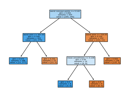

We could count the leaves, or query best_ instead.

best_.tree_.n_leaves

from sklearn.metrics import accuracy_score, mean_squared_error
print('Accuracy Train' , best_.score(X_train, y_train).round(2) ) 
print('Accuracy Test' , best_.score(X_test, y_test).round(2) ) 
print( 'Test MSE:', mean_squared_error(y_test, best_.predict(X_test)).round(2) )

Accuracy Train 0.96
Accuracy Test 0.97
Test MSE: 0.03

Code

from ISLP import load_data, confusion_table

confusion = confusion_table(best_.predict(X_test), y_test)
confusion

Table 3: Confusion Matrix

Truth	0	1
Predicted
0	45	1
1	2	66

Pruning the tree clearly help the performance of our tree classifier.

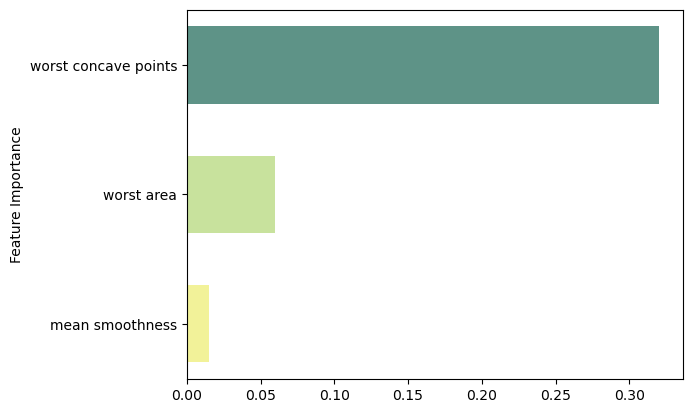
Feature Importance

feat_importance = best_.tree_.compute_feature_importances(normalize=False)
column_names = df.drop(columns='target').columns.tolist()

fimp_df = pd.DataFrame(feat_importance, column_names).reset_index().sort_values(0, ascending=False).head(3)

Code

fig, ax = plt.subplots()

# Setup
data = fimp_df.loc[:,0].sort_values()
index = np.arange(data.shape[0])
bar_labels = fimp_df.sort_values(0).loc[:,'index'].tolist()
bar_colors = ['#F2F299', '#C8E29D', '#5E9387', '#58828B']
bar_width = 0.6

# Figure
ax.barh(index, data, bar_width, label=bar_labels, color=bar_colors)

# Labels
ax.set_ylabel('Feature Importance')
ax.set_yticks(index, labels=bar_labels)

# Show
plt.show()

Figure 6: Feature Importance Regression Tree