import numpy as np
import pandas as pd
import matplotlib.pyplot as plt
import seaborn as sns

import warnings
warnings.filterwarnings("ignore")Model Evaluation Rules: Cross Validation
Once a predictive model (classifier or regressor) is constructed, it is particularly important to evaluate its performance. Model evaluation stage include the use of methods and metrics to estimate the predictive performance of a model. To understand the model evaluation process, it would be helpful to distinguish between evaluation rules and evaluation metrics.
- A evaluation metric is used to quantify the performance of a constructed model.
- A model evaluation rule, on the other hand, refers to the procedure that is used to estimate a metric. In other words, a metric could be estimated using various rules.
For simplicity of discussion, in what follows, estimation rules are described in connection with classification error rate. However, all procedures, except when stated otherwise, are applicable to estimating classifier and regressor performance metrics.
For more, check here: https://scikit-learn.org/stable/model_selection.html#model-selection
Hold-Out Estimator
Suppose that we would like to estimate the test error associated with fitting a particular statistical learning method on a set of observations. The Hold-Out Approach is a very simple strategy validation set approach for this task:

It involves randomly dividing the available set of observations into two parts, a training set and a validation set or hold-out set.
The model is fit on the training set, and the fitted model is used to predict the responses for the observations in the validation set.
The validation set approach is conceptually simple and is easy to implement. But it has two potential drawbacks:
- Results can be highly variable, depending which observations are included in the training set.
- Only a subset of the observations are used to fit the model.
Application with train_test_split
Let’s go back to our kNN classifier example:
Code
from sklearn import datasets
iris = datasets.load_iris()

df = pd.DataFrame(iris.data, columns=iris.feature_names)
# Add target
df['target'] = iris.target

# Dictionary
target_names_dict = {0: 'setosa', 1: 'versicolor', 2: 'virginica'}

# Add the target names column to the DataFrame
df['target_names'] = df['target'].map(target_names_dict)
df.head(5)| sepal length (cm) | sepal width (cm) | petal length (cm) | petal width (cm) | target | target_names | |
|---|---|---|---|---|---|---|
| 0 | 5.1 | 3.5 | 1.4 | 0.2 | 0 | setosa |
| 1 | 4.9 | 3.0 | 1.4 | 0.2 | 0 | setosa |
| 2 | 4.7 | 3.2 | 1.3 | 0.2 | 0 | setosa |
| 3 | 4.6 | 3.1 | 1.5 | 0.2 | 0 | setosa |
| 4 | 5.0 | 3.6 | 1.4 | 0.2 | 0 | setosa |
In scikit-learn a random split into training and test sets can be quickly computed with the train_test_split helper function. For example, we can now quickly sample a training set while holding out 40% of the data for testing (evaluating) our classifier:
from sklearn.model_selection import train_test_split
from sklearn.preprocessing import StandardScaler
from sklearn.neighbors import KNeighborsClassifier as kNN

# Target vs Inputs
X = df.drop(columns=["target", "target_names"]) # Covariates-Only
y = df["target"] # Target-Outcome

# Train vs Split
X_train, X_test, y_train, y_test = train_test_split(X, y, stratify=y, test_size=0.4, random_state=0)

# Normalization
scaler = StandardScaler()
X_train = scaler.fit_transform(X_train)
X_test = scaler.transform(X_test)

# Instantiate Class into Object. Set Parameters
knn = kNN(n_neighbors=3)

# Train Model
knn.fit(X_train, y_train)

# Predict
y_test_pred = knn.predict(X_test)
To calculate the test error on the held-out data, we just use the score function.
Note that each estimator have a default score method providing a evaluation criterion for the problem they are designed to solve.
from sklearn.metrics import accuracy_score, mean_squared_error
print('Accuracy Train', knn.score(X_train, y_train).round(2) )
print('Accuracy Test', knn.score(X_test, y_test).round(2) )
Accuracy Train 0.94
Accuracy Test 0.97k-Fold Cross Validation
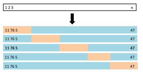
The k-fold CV approach involves randomly dividing the set of observations into k groups, or folds, of approximately equal size. The first fold is treated as a validation set, and the method is fit on the remaining k − 1 folds.
- The mean squared error, \text{MSE}_1, is then computed on the observations in the held-out fold.
- This procedure is repeated k times; each time, a different group of observations is treated as a validation set.

This process results in k estimates of the test error, \text{MSE}_1,...,\text{MSE}_k . The k-fold CV estimate is computed by averaging these values:
\text{CV}_k=\frac{1}{k}\sum^k_{i=1}\text{MSE}_k
- It is not hard to see that LOOCV is a special case of k-fold CV in which k is set to equal n.
It is important to keep in mind that cross-validation does not return a model. When calling cross_val_score, multiple models are built internally, but the purpose of cross-validation is only to evaluate how well a given algorithm will generalize when trained on a specific dataset.
Application: cross_validate and cross_val_score
The simplest way to use cross-validation is to call the cross_val_score helper function on the estimator and the dataset. Lets create k=10 folds:
from sklearn.neighbors import KNeighborsClassifier as kNN
from sklearn.model_selection import cross_val_score

# Instantiate Class into Object. Set Parameters
knn = kNN(n_neighbors=3)

# Train Model with K-Fold
scores = cross_val_score(knn, X, y, cv=10)
print("Cross-validation scores: {}".format(scores))

# Mean Score
print( 'Mean Score (Accuracy):', scores.mean().round(2) )
Cross-validation scores: [1. 0.93333333 1. 0.93333333 0.86666667 1.
0.93333333 1. 1. 1. ]
Mean Score (Accuracy): 0.97Splitting the dataset into k folds by starting with the first one-k-th part of the data might not always be a good idea.
By default, scikit-learn does not use it for classification, but rather uses stratified k-fold cross-validation. In stratified cross-validation, we split the data such that the proportions between classes are the same in each fold.
model_selection.cross_val_score take a scoring parameter that controls what metric they apply to the estimators evaluated. By default, the score computed at each CV iteration is the score method of the estimator. It is possible to change this by using the scoring parameter:
# Train Model with K-Fold
scores = cross_val_score(knn, X, y, cv=10, scoring='f1_macro')

# Mean Score
print( 'Mean Score:', scores.mean().round(2) )
Mean Score: 0.97Alternatively, there is the cross_validate function, which differs a bit from cross_val_score in two ways:
- It allows specifying multiple metrics for evaluation.
- It returns a dict containing
fit-times,score-timesin addition to thetest score.
from sklearn.neighbors import KNeighborsClassifier as kNN
from sklearn.model_selection import cross_validate

# Instantiate Class into Object. Set Parameters
knn = kNN(n_neighbors=3)

# Cross validation and performance evaluation
knn_score = cross_validate(knn, X, y, cv=10)

# Mean Score
print('Mean Score:', knn_score["test_score"].mean().round(2) )

# Scores
knn_score = pd.DataFrame(knn_score)
knn_score.head(3)
Mean Score: 0.97| fit_time | score_time | test_score | |
|---|---|---|---|
| 0 | 0.005152 | 0.005557 | 1.000000 |
| 1 | 0.003806 | 0.004162 | 0.933333 |
| 2 | 0.003748 | 0.003971 | 1.000000 |
# Call Multiple Metrics
scoring = ['precision_macro', 'recall_macro']
knn_score = cross_validate(knn, X, y, cv=10, scoring=scoring)
pd.DataFrame(knn_score).head(4)| fit_time | score_time | test_precision_macro | test_recall_macro | |
|---|---|---|---|---|
| 0 | 0.004226 | 0.011323 | 1.000000 | 1.000000 |
| 1 | 0.002567 | 0.007165 | 0.944444 | 0.933333 |
| 2 | 0.001993 | 0.006492 | 1.000000 | 1.000000 |
| 3 | 0.002992 | 0.006701 | 0.944444 | 0.933333 |
Leave-One-Out Cross Validation (LOOCV)
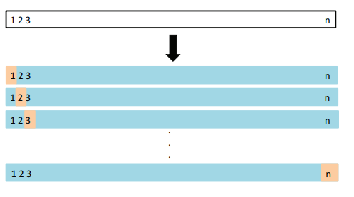
In LOOCV, a single observation (x_1, y_1) is used for the validation set, and the remaining observations [(x_2, y_2),...,(x_n, y_n)] make up the training set.
- The statistical learning method is fit on the n − 1 training observations, and a prediction \hat{y}_1 is made for the excluded observation, using its value x_1.
- Since (x_1, y_1) was not used in the fitting process, \text{MSE}_1 = (y_1 − \hat{y}_1)^{2} provides an approximately unbiased estimate for the test error.
- But even though \text{MSE}_1 is unbiased for the test error, it is a poor estimate because it is highly variable, since it is based upon a single observation (x_1, y_1).
Solution: We can repeat the procedure by selecting (x_2, y_2) for the validation data, training the statistical learning procedure on the n − 1 observations [(x_1, y_1),(x_3, y_3),...,(x_n, y_n)], and computing \text{MSE}_2=(y_2-\hat{y}_2)^2.

- Repeating this approach n times produces n squared errors, \text{MSE}_1,..., \text{MSE}_n.
The LOOCV estimate for the test MSE is the average of these n test error estimates:
\text{CV}_n=\frac{1}{n}\sum^n_{i=1}\text{MSE}_i
Application with LeaveOneOut
from sklearn.model_selection import LeaveOneOut

loo = LeaveOneOut()

scores = cross_val_score(knn , X, y, cv=loo)

print("Number of cv iterations: ", len(scores))
print("Mean accuracy: {:.2f}".format(scores.mean()))
Number of cv iterations: 150
Mean accuracy: 0.96