Model Evaluation Metrics

import numpy as np
import pandas as pd
import matplotlib.pyplot as plt
import seaborn as sns

import warnings
warnings.filterwarnings("ignore")

There are 3 different APIs for evaluating the quality of a model’s predictions:

1. Estimator default’s score method: Estimators have a score method providing a default evaluation criterion for the problem they are designed to solve.
2. Scoring parameter: Model-evaluation tools using cross-validation (such as model_selection.cross_val_score and model_selection.GridSearchCV) rely on an internal scoring strategy.
3. Metric functions: The sklearn.metrics module implements functions assessing prediction error for specific purposes. These metrics are detailed in sections.

1. Classification Metrics with sklearn.metrics

Our aim here is to use an evaluation rule to estimate the performance of a trained classifier. In this section, we will cover different metrics to measure various aspects of a classifier performance.

The sklearn.metrics module implements several loss, score, and utility functions to measure classification performance: - Accuracy: accuracy_score(y_true, y_pred) - Confusion Matrix: confusion_matrix(y_true, probas_pred) - Recall: recall_score(y_true, probas_pred) - Precision: precision_score(y_true, probas_pred) - $F_1$ Score: f1_score(y_true, y_pred)

from sklearn import datasets
iris = datasets.load_iris()

df = pd.DataFrame(iris.data, columns=iris.feature_names)
# Add target
df['target'] = iris.target

# Dictionary
target_names_dict = {0: 'setosa', 1: 'versicolor', 2: 'virginica'}

# Add the target names column to the DataFrame
df['target_names'] = df['target'].map(target_names_dict)
df.head(5)

Table 1: Iris Dataset

	sepal length (cm)	sepal width (cm)	petal length (cm)	petal width (cm)	target	target_names
0	5.1	3.5	1.4	0.2	0	setosa
1	4.9	3.0	1.4	0.2	0	setosa
2	4.7	3.2	1.3	0.2	0	setosa
3	4.6	3.1	1.5	0.2	0	setosa
4	5.0	3.6	1.4	0.2	0	setosa

from sklearn.model_selection import train_test_split
from sklearn.preprocessing import StandardScaler
from sklearn.neighbors import KNeighborsClassifier as kNN

# Target vs Inputs
X = df.drop(columns=["target", "target_names"]) # Covariates-Only
y = df["target"] # Target-Outcome

# Train vs Split
X_train, X_test, y_train, y_test = train_test_split(X, y, stratify=y, test_size=0.4, random_state=0)

# Normalization
scaler = StandardScaler()
X_train = scaler.fit_transform(X_train) 
X_test = scaler.transform(X_test) 

# Instantiate Class into Object. Set Parameters
knn = kNN(n_neighbors=3)

# Train Model
knn.fit(X_train, y_train)

# Predict
y_test_pred = knn.predict(X_test)

1.1. Accuracy, Precision, Recall in sklearn.metrics

For multiclass classification (such as this example), functions such as precision_score and recall_score supports average=['macro', 'weighted', 'micro'].

• If we set average="None" to print these metrics for each class individually (when the class is considered positive).

from sklearn.metrics import accuracy_score, precision_score, recall_score
print('Accuracy Score', accuracy_score(y_test, y_test_pred).round(2) ) 
print('Precision Score (Macro)', precision_score(y_test, y_test_pred, average='macro').round(2) ) 
print('Recall Score (Macro)', recall_score(y_test, y_test_pred, average='macro').round(2) ) 

Accuracy Score 0.97
Precision Score (Macro) 0.97
Recall Score (Macro) 0.97

1.2. Confusion Matrix Display

The confusion_matrix function evaluates classification accuracy by computing the confusion matrix with each row corresponding to the true class (Wikipedia and other references may use different convention for axes).

from sklearn.metrics import confusion_matrix, ConfusionMatrixDisplay
y_true = [0, 0, 0, 1, 1, 1, 1, 1, 0, 0]
y_pred = [0, 1, 0, 1, 0, 1, 0, 1, 0, 0]
confusion_matrix(y_true, y_pred, normalize='all')

array([[0.4, 0.1],
       [0.2, 0.3]])

ConfusionMatrixDisplay can be used to visually represent a confusion matrix as shown in the Confusion matrix example, which creates the following figure:

cm = confusion_matrix(y_true, y_pred)
disp = ConfusionMatrixDisplay(confusion_matrix=cm)
disp.plot(cmap='magma')
plt.show()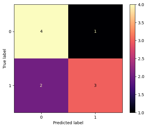

Figure 1: Confusion Matrix Results

• The parameter normalize allows to report ratios instead of counts.
• The confusion matrix can be normalized in 3 different ways: pred, true, and all which will divide the counts by the sum of each columns, rows, or the entire matrix, respectively.
• The cmap controls in .plot() defines the color palette. default is viridis. Others are magma, plasma, mako, inferno.

1.3. Metrics using scoring from sklearn.model_selection

In order to use one of the aforementioned metrics along with cross-validation, we can set the scoring parameter of cross_validate or cross_val_score to a string that represents the metric.

Model selection and evaluation using tools, such as model_selection.cross_val_score and model_selection.GridSearchCV, take a scoring parameter that controls what metric they apply to the estimators evaluated.

The following list below shows some common possible values.

For Classification:

• ‘accuracy’: metrics.accuracy_score
• ‘precision’: metrics.precision_score
• ‘recall’: metrics.recall_score
• ‘f1_macro’: metrics.f1_score
• ‘roc_auc’: metrics.roc_auc_score

cross_validate

from sklearn.neighbors import KNeighborsClassifier as kNN
from sklearn.model_selection import cross_validate

# Instantiate Class into Object. Set Parameters
knn = kNN(n_neighbors=3)

# Call Multiple Metrics
scoring = ['accuracy', 'precision_macro', 'recall_macro', 'roc_auc_ovr', 'r2', 'neg_mean_squared_error']

# Cross validation and performance evaluation
knn_score = cross_validate(knn, X, y, cv=5, scoring=scoring) 

# Scores
knn_score = pd.DataFrame(knn_score)
knn_score

	fit_time	score_time	test_accuracy	test_precision_macro	test_recall_macro	test_roc_auc_ovr	test_r2	test_neg_mean_squared_error
0	0.003936	0.018189	0.966667	0.969697	0.966667	0.973333	0.95	-0.033333
1	0.002517	0.014405	0.966667	0.969697	0.966667	1.000000	0.95	-0.033333
2	0.001958	0.016940	0.933333	0.944444	0.933333	0.990000	0.90	-0.066667
3	0.001999	0.016462	0.966667	0.969697	0.966667	0.971667	0.95	-0.033333
4	0.003011	0.013062	1.000000	1.000000	1.000000	1.000000	1.00	-0.000000

2. Regression Metrics in sklearn.metrics

Our aim now is to estimate the predictive ability of the regressor. We will apply the three most common metrics: MSE, RMSE, MAE, and R2, also known as coefficient of determination.

The sklearn.metrics module implements several loss, score, and utility functions to measure regression performance. Some of those have been enhanced to handle the multi-output case:

• MSE: mean_squared_error(y_true, y_pred)
• RMSE: mean_root_squared_error(y_true, y_pred)
• MAE: mean_absolute_error(y_true, y_pred)
• $R^2$: r2_score(y_true, y_pred)

2.1. Metrics using scoring from sklearn.model_selection

Model selection and evaluation using tools, such as model_selection.cross_val_score and model_selection.GridSearchCV, take a scoring parameter that controls what metric they apply to the estimators evaluated.

The following list below shows some common possible values.

For Regression:

• ‘neg_mean_squared_error’: metrics.mean_squared_error
• ‘neg_root_mean_squared_error’: metrics.root_mean_squared_error
• ‘r2’: metrics.r2_score

Important Note: All scorer objects follow the convention that higher return values are better than lower return values. Thus metrics such as metrics.mean_squared_error are here available as neg_mean_squared_error which return the negated value of the metric.